Recovered equations and ordinates of the Göttingen 765 airfoil

by Keith Pickering

Symbols

a₀, a₁, a₂, a₃ Coefficients of forebody thickness distribution

d₀, d₁, d₂, d₃ Coefficients of afterbody thickness distribution

h Principal component coefficient

I Leading edge sharpness parameter

m Position of maximum thickness as a fraction of chord

m_n Nominal meanline

m_e Empirical meanline

r_LE Leading edge radius

T Airfoil thickness as a fraction of chord

x A position along airfoil chord

x_u Upper surface x ordinate

x_l lower surface x ordinate

y A distance above or below airfoil chord

y_l lower surface y ordinate

y_t thickness distribution at given x

y_u upper surface y ordinate

y_P Meanline principal component

y_S Meanline sigmoid component

y_R Meanline residual component

λ Sigmoid component coefficient

θ Angle of meanline slope

Introduction

The Göttingen 765 is known as the root-section airfoil of the Me163 Komet, a rocket-powered tailless interceptor of WWII fame. But no definitive ordinates of the Göttingen 765 exist. While surviving drawings and museum examples provide low-resolution data on the shape of the airfoil, it is often useful to have more exact equations of the ordinates for research purposes. Here we derive a meanline and thickness distribution that fit these measurements.

The meanline

The shape of the meanline is particularly important, because like all tailless aircraft the Me163 requires a wing that has a coefficient of moment that is both close to zero, and stable through a wide range of angles of attack. The papers of Alexander Lippisch, chief designer of the Me163, are at Iowa State University in Ames. Among them is a graph showing the camber line of the Göttingen 765 and four other similar airfoils, differing by the amount of reflex at the trailing edge (De Bie 2000). Although there are no equations given for camber lines on the drawing, Borst 1980 states that the meanline for the Göttingen 765 is the sum of these two equations:

(1)

(2)

where m and n are integers. Although the values of h, λ, m, and n are not given, it is possible to recover the values of those coefficients using multiple regression against the ISU curve. A very close fit occurs where m=2, n=2, h=0.00573952678, and λ=0.018521412. But Lippisch, working with only a slide rule, could not have carried more than two or “two-and-a-half” significant digits into any calculation. Rounding to that precision gives us h=.00575 and λ=.0185. The Borst meanline then becomes

(3)

and differentiating gives

(4)

Equations 3 and 4 can be used to generate a nominal airfoil by wrapping the standard NACA 4-digit thickness distribution around the Borst meanline, given the known thickness of the airfoil (14.4% of chord). Since the NACA distribution was originally derived by reference to the Göttingen 398 airfoil (Jacobs et. al. 1933), it stands to reason that the thickness distribution of the 765 should be at least somewhat similar to NACA's standard. That thickness distribution is given by the well-known equation:

(5)

For any given position on the chord (0 ≤ x ≤ 1) ordinates of the upper and lower surface can be generated as follows: y_t values for the given x are found from equation 5; the meanline m_n for x is found from equation 3, and its slope is found from equation 4. The slope angle θ is simply . Then ordinates for the upper surface are ; ; and for the lower surface are; .

This computed airfoil can be compared to the actual Göttingen 765. Ordinates for the airfoil can be found at De Bie 2000, in several versions. The highest quality and best-measured version is one made from a Messerschmitt factory drawing, which I will take as standard in this paper. Figure 1 is a foreshortened graph showing this profile against the profile just computed.

Figure 1. Foreshortened plot of the Messerschmitt factory drawing compared to computed profile. Errors are clearly present.

It is clear from figure 1 that the computed airfoil, though vagely similar to the Göttingen 765, has a large flaw in the middle section, where the computed profile shows less camber than the actual airfoil. This can only be due to an error in the Borst meanline, implying that both the ISU curve and Borst 1980 are not fully correct in their treatment of the meanline. It may well be that the originally intended meanline was modified after wind tunnel testing showed a need for increased camber. If that is the case, it is possible that surviving documentation reflects the original meanline rather than the one used in the actual aircraft.

To investigate this further, I found y-ordinates for the computed airfoil corresponding to the x-ordinates for each point in the De Bie dataset. By subtracting the computed airfoil y-ordinates from the y-ordinates of the drawing, a set of residual values can be obtained. These residuals are shown in figure 2.

Figure 2. Residuals of the y-ordinates, using the Borst meanline and NACA-4 digit thickness.

The mid-chord flaw shows up clearly as a large hump in this figure. Note also that, if our thickness distribution were incorrect it would show up in figure 2 as a gap between the residuals of the upper and lower surfaces. In both cases, those gaps are generally small except at the leading and trailing edges.

Notice too that at the leading edge, the De Bie dataset has significantly smaller ordinates (less apparent camber) than the computed airfoil. This is almost certainly an artifact of measurement, since the exact point of an airfoil's leading edge chord is often difficult to determine by eye. To correct this, we rotate the ordinates of the De Bie data around the trailing edge clockwise by .0048 radian, so the residuals near the leading edge come close to zero. Re-drawing the residuals after this rotation gives us a residual dataset that is nearly zero at both leading and trailing edges (figure 3), which is what we want.

Figure 3. Same as figure 2, with drawing rotated .0048 radian clockwise around trailing edge.

The reason for the rotation is that we would like to flatten that hump. To do that, we need to add a new constituent equation to the meanline that will reduce these residuals to reasonably low values. But any meanline must cross the axis at x=0 and x=1, which means the only way to correct residuals at those points is by rotation. Those few datapoints at the very leading edge, which show great disparities from the computed airfoil, are an artifact of the way the drawing was measured; since the profile is nearly vertical at the leading edge, slight errors in measuring the x-ordinate result in spuriously large errors in the y-ordinate. These residuals can be safely ignored. Again we use multiple regression to find an equation that fits the residual data closely, constraining coefficients so that y=0 at x=1, x=0. In this case rounding to sliderule precision is not adequate for the task, but using slightly more precision we find:

(6)

Combining equations 3 and 6 gives us the empirical meanline:

(7)

and differentiating gives

(8)

This meanline has a maximum camber of .019 at 26% of chord. Following the same procedure as before, we wrap the NACA 4-digit thickness distribution around the empirical meanline and derive a “first cut” empirical version of the Göttingen 765. Comparing this to figure 3 shows that we have indeed corrected the camber.

Figure 4. Residuals after adding empirical correction to the Borst meanline.

The thickness distribution

Plotting the residuals of the empirical airfoil to the De Bie dataset shows problem areas in a small slice of the extreme leading edge, and a broader region of the trailing edge. In both cases, the empirical airfoil is too thick, causing the upper-surface and lower-surface residuals to diverge.

The standard NACA 4-digit distribution has a small gap at the trailing edge, amounting to about 1% of the airfoil thickness. It is clear from the residual plot that this gap is responsible for the large residual at the trailing edge. Therefore the thickness distribution must be modified. A procedure for generating modified thickness distributions can be found in Stack and Von Doenhoff 1934. In addition to the trailing edge gap, there are three other parameters that can be varied by this procedure: the trailing edge angle; the leading edge radius; and m, the position of maximum thickness. Specifying the trailing edge gap and slope provides two of the four coefficients we need for the thickness distribution.

(9)

For our purposes, we set d₀=0 to close the trailing edge gap entirely. Next,

d₁ = Trailing edge slope (10)

Stack & Von Doenhoff have provided a table with suggested values for the trailing edge slope based on the position of maximum thickness m=x, chosen to avoid a reflexive surface. The standard value of m=.3 is correct for the Göttingen 765.

m	d1
.2	1.000 T
.3	1.170 T
.4	1.575 T
.5	2.325 T
.6	3.500 T

Here T is thickness expressed as a fraction of the chord. If other positions of m are desired, the figures in this table are closely replicated by

(11)

Since m=.3 is correct, we provisionally adopt d₁=1.170T = .16848. Then,

(12)

and

(13)

These four parameters set the thickness distribution aft of the point of maximum thickness. Forward of that point, we define an index parameter I that controls the leading edge radius and the thickness of the nose. In the standard case I=6 but this can be modified within the range 0 ≤ I < 9. Brief experimentation shows that I=5.7 gives a nearly perfect fit to the nose of the airfoil (and is much superior to the standard NACA 4-digit distribution).

Then, following Mason 1995, we compute the following:

(14)

(15)

(16)

(17)

(18)

The leading edge radius is given by

(19)

Finally, the thickness distribution ahead of the maximum thickness point x=m is found by

(20)

and aft of the maximum thickness point by

(21)

Since this is different from the standard NACA 4-digit distribution, we can expect the residual plot to change too; and the changes are particularly beneficial to the leading and trailing edges. In fact, the fit is so close that there can be little doubt that the NACA modified distribution was in fact the distribution used in the Göttingen 765. As far as I am aware, this is the only known case of the NACA modified 4-digit thickness distribution being used in a German aircraft of WWII.

Figure 5. Residuals after applying modified thickness distribution to the empirical meanline.

Looking at the final residual plot (figure 5), both surfaces of our recovered airfoil are within .001 of the Messerschmitt drawing for nearly the entire length. The leading edge area is particularly well fit. Only the trailing edge upper surface continues to show a discrepancy, from 75% of the chord back, where the Messerschmitt drawing is slightly thicker than our recovered version. It appears as if the slightly reflexive surface at this point has been flattened; this may be due to slight modifications needed for control surfaces. It is possible to remove that trailing edge discrepancy by increasing the trailing edge slope parameter d₁, but that creates a bigger problem that it solves farther forward, when the recovered version becomes noticeably thicker than the drawn version.

Figure 6. Scale drawing of final recovered airfoil.

Appendix A.

Ordinates for the recovered Göttingen 765 airfoil.

Göttingen 765 airfoil (recovered). Thick: .144 LE radius: 0.02062 LE slope: 0.17300

1.000000 -0.000000

0.989894 0.000681

0.979818 0.001451

0.969768 0.002306

0.959744 0.003241

0.949742 0.004251

0.939760 0.005332

0.929797 0.006480

0.919852 0.007690

0.909921 0.008959

0.900004 0.010282

0.890099 0.011656

0.880204 0.013078

0.870319 0.014543

0.860440 0.016049

0.850569 0.017592

0.840702 0.019170

0.830839 0.020778

0.820980 0.022415

0.811122 0.024076

0.801265 0.025760

0.791409 0.027463

0.781551 0.029184

0.771693 0.030918

0.761832 0.032664

0.751969 0.034419

0.742102 0.036181

0.732232 0.037948

0.722357 0.039717

0.712477 0.041485

0.702591 0.043251

0.692701 0.045013

0.682804 0.046768

0.672900 0.048514

0.662990 0.050250

0.653073 0.051973

0.643149 0.053681

0.633218 0.055373

0.623278 0.057046

0.613331 0.058699

0.603376 0.060330

0.593413 0.061938

0.583441 0.063519

0.573461 0.065074

0.563472 0.066599

0.553475 0.068093

0.543469 0.069555

0.533454 0.070983

0.523430 0.072376

0.513397 0.073731

0.503355 0.075047

0.493303 0.076322

0.483243 0.077555

0.473172 0.078745

0.463093 0.079889

0.453003 0.080986

0.442904 0.082034

0.432796 0.083032

0.422677 0.083979

0.412549 0.084871

0.402410 0.085709

0.392262 0.086490

0.382103 0.087212

0.371934 0.087874

0.361755 0.088474

0.351565 0.089011

0.341365 0.089482

0.331155 0.089885

0.320934 0.090220

0.310703 0.090484

0.300461 0.090675

0.290208 0.090785

0.279946 0.090803

0.269673 0.090725

0.259390 0.090547

0.249098 0.090261

0.238797 0.089864

0.228488 0.089348

0.218172 0.088708

0.207849 0.087937

0.197522 0.087028

0.187191 0.085974

0.176858 0.084767

0.166525 0.083397

0.156195 0.081855

0.145870 0.080131

0.135554 0.078212

0.125250 0.076086

0.114964 0.073738

0.104700 0.071149

0.094465 0.068300

0.084267 0.065166

0.074117 0.061714

0.064025 0.057907

0.054009 0.053690

0.044090 0.048989

0.039176 0.046425

0.034298 0.043693

0.029464 0.040768

0.024683 0.037614

0.019965 0.034182

0.015330 0.030393

0.010806 0.026119

0.006448 0.021104

0.002392 0.014696

-0.000000 0.000000

0.007608 -0.012992

0.013552 -0.017745

0.019194 -0.021153

0.024670 -0.023870

0.030035 -0.026149

0.035317 -0.028118

0.040536 -0.029854

0.045702 -0.031406

0.050824 -0.032810

0.055910 -0.034090

0.065991 -0.036349

0.075975 -0.038289

0.085883 -0.039981

0.095733 -0.041470

0.105535 -0.042792

0.115300 -0.043972

0.125036 -0.045030

0.134750 -0.045983

0.144446 -0.046843

0.154130 -0.047620

0.163805 -0.048323

0.173475 -0.048960

0.183142 -0.049537

0.192809 -0.050060

0.202478 -0.050534

0.212151 -0.050962

0.221828 -0.051349

0.231512 -0.051699

0.241203 -0.052014

0.250902 -0.052297

0.260610 -0.052551

0.270327 -0.052779

0.280054 -0.052981

0.289792 -0.053162

0.299539 -0.053322

0.309297 -0.053469

0.319066 -0.053609

0.328845 -0.053740

0.338635 -0.053862

0.348435 -0.053973

0.358245 -0.054075

0.368066 -0.054164

0.377897 -0.054242

0.387738 -0.054306

0.397590 -0.054358

0.407451 -0.054395

0.417323 -0.054417

0.427204 -0.054424

0.437096 -0.054414

0.446997 -0.054388

0.456907 -0.054345

0.466828 -0.054283

0.476757 -0.054203

0.486697 -0.054104

0.496645 -0.053984

0.506603 -0.053844

0.516570 -0.053683

0.526546 -0.053500

0.536531 -0.053295

0.546525 -0.053066

0.556528 -0.052813

0.566539 -0.052535

0.576559 -0.052232

0.586587 -0.051903

0.596624 -0.051546

0.606669 -0.051161

0.616722 -0.050748

0.626782 -0.050305

0.636851 -0.049831

0.646927 -0.049325

0.657010 -0.048787

0.667100 -0.048215

0.677196 -0.047607

0.687299 -0.046964

0.697409 -0.046284

0.707523 -0.045565

0.717643 -0.044806

0.727768 -0.044006

0.737898 -0.043163

0.748031 -0.042276

0.758168 -0.041343

0.768307 -0.040363

0.778449 -0.039333

0.788591 -0.038253

0.798735 -0.037121

0.808878 -0.035934

0.819020 -0.034690

0.829161 -0.033388

0.839298 -0.032026

0.849431 -0.030600

0.859560 -0.029110

0.869681 -0.027552

0.879796 -0.025925

0.889901 -0.024225

0.899996 -0.022451

0.910079 -0.020600

0.920148 -0.018668

0.930203 -0.016654

0.940240 -0.014555

0.950258 -0.012367

0.960256 -0.010088

0.970232 -0.007715

0.980182 -0.005244

0.990106 -0.002674

1.000000 -0.000000

Appendix B.

Polars for the recovered Göttingen 765 airfoil. Data generated with XFOIL, n_crit=9.

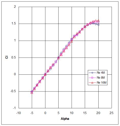
Figure A-1. Angle of attack vs. coefficient of lift.

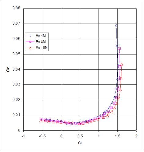
Figure A-2. Coefficient of lift vs. coefficient of drag.

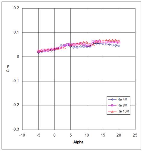
Figure A-3. Angle of attack vs. coefficient of moment.

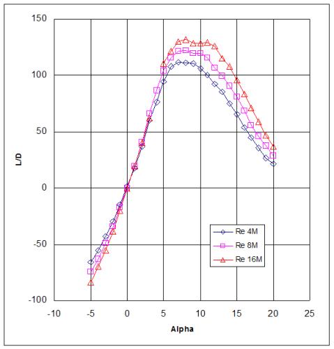
Figure A-4. Angle of attack vs. Lift/Drag ratio.

References

Borst, Henry V. (1980). The Aerodynamics of the Unconventional Air Vehicles of A. Lippisch. Self-published, ISBN 978-1570874277.

De Bie, Rob (2000). Me163 Profiles. http://robdebie.home.xs4all.nl/me163/profiles.htm (accessed 2012/3/13).

Jacobs, Eastman N, Ward, Kenneth E, and Pinkerton, Robert M. (1933) The characteristics of 78 related airfoil sections from tests in the variable-density wind tunnel. NACA report 460.

Mason, W. H. (1995). Applied Computational Aerodynamics, Appendix A: Geometry for aerodynamicists. http://www.dept.aoe.vt.edu/~mason/Mason_f/CAtxtTop.html (accessed 2012/3/13).

Stack, John and Von Doenhoff, Albert (1934) Tests of 16 related airfoils at high speeds. NACA report 492.